1  Categories, Morphisms, and Diagrams

1.1 Motivation

Discussion 1.1.1. A category is a collection of mathematical objects of one type along with directed relationships between those objects. Category theory forces us to step back and make sure we understand the context in which we are working. When we meet a mathematical object, before we dive into details, we should pause to ask what type of object it is. Is it a set, a topological space, a vector space, etc? What are the relationships that matter in this context?

The directed relationships between objects in categories will go by several names — maps, arrows, or morphisms will be used freely and interchangeably. These maps carry directionality by having a start and an end. They will begin with an object (the source or domain) and end in some object (the target or codomain). We will depict them graphically in diagrams such as \(X \xrightarrow{f} Y\) where \(f\) is the map starting at object \(X\) and ending at object \(Y\).

A philosophy that we will emphasize constantly is that an object is understood precisely via understanding all the maps into and out of that object. We take as a working slogan that mathematical structure is precisely whatever is mapped, detected, preserved, or collapsed by maps into or out of the objects in question. Consequently, whenever we meet a new mathematical object we will immediately ask what the “right” sort of map is for that object, because it is through maps that we will learn about the object.

Looking ahead to the next chapter, we will introduce another recurring pattern, where we shift from starting with objects and asking about maps to starting with maps and asking about objects. In particular, we will describe a general process of packaging a problem as a map and then seeking a particular object that, in a special way, characterizes that mapping. That general pattern will be used repeatedly later in the book and lead to several of the most important objects we will study. Objects matter in math, but often it is maps that characterize the objects and serve as the reason why the objects are important in the first place.

The rest of this chapter will:

• Define categories and give some examples that may or may not yet make sense.

• Present commutative diagrams, which will pervade much of our exposition, and highlight the need for the reader to become fluent in the equivalent dialects of diagrams, equations, and statements.

• Describe switching perspectives on a category to give opposite categories, a crucial ingredient throughout math.

• Describe the probing philosophy we will adopt.

• Present the categorical notion of sameness — isomorphisms.

• Delve into two other faithful probes, monomorphisms & epimorphisms.

• Define initial, terminal, & zero objects.

• Describe elements and generalized elements.

• Discuss Hom sets.

• Finally, synthesize the material and look ahead to maps between categories (functors).

Everything in this chapter should be read before proceeding, although much of it may only sink in after progressing further in the book and then returning to these ideas with more context and experience.

1.2 Defining a Category

Discussion 1.2.1. Strictly speaking, definitions are not something we derive but something we define. Be that as it may, often in mathematics we do partially derive fitting definitions. It works like this: we have a problem of interest in some sort of context. This context and details of the problem force some sort of constraints on what we consider. Our definitions then end up as whatever satisfies the constraints with no additional constraints imposed. This derivation is not logically necessary like logical derivations in a proof, but is essential as good definitions focus our attention on the right structures and bad definitions fail to capture the important parts of a problem (or capture them, but add extra, extraneous details). In actual mathematical practice, it can take a long time to acquire the skill to craft good definitions, and, even for a skilled practitioner, it can only be in hindsight that we see clearly which definitions hit the mark.

Our task in this section is to come up with a sensible definition of a category. Generically, we need a sensible way to talk about a class of mathematical objects of one type that are related to each other in a directional way. Our problem immediately fixes a couple things.

First, a category \(\mathcal{A}\) will have to have objects, these being the mathematical things in question. We will sometimes write \(\mathop{\mathrm{ob}}(\mathcal{A})\) for the objects of category \(\mathcal{A}\) and write \(X \in \mathop{\mathrm{ob}}(\mathcal{A})\) or even \(X \in \mathcal{A}\) to show \(X\) is an object in \(\mathcal{A}\). (Note, parenthetically, that categories can be small with a finite number of objects or so massive they are not sets. So when we write \(X \in \mathcal{A}\) we are not necessarily asserting that the objects of category \(\mathcal{A}\) form a set; we are abusing notation from sets for convenience.)

We want our mathematical objects to be relatable in a directed way. This desire is not necessarily transparent from the outset, but take it as part of our motivation that we want relationships between objects where the relationship starts somewhere (in some object) and ends somewhere (in some object). So, for objects \(X, Y \in \mathcal{A}\) (we are colloquially saying \(X\) and \(Y\) are objects of \(\mathcal{A}\) with the notation \(X, Y \in \mathcal{A}\)), we pictorially depict a relation from \(X\) to \(Y\) with an arrow: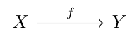

We will call these arrows or maps or morphisms (or directed relationships). The start of an arrow is its source or domain. The end of an arrow is its target or codomain.

Importantly, we will not just care about single maps, but all maps between pairs of objects. For objects \(X, Y \in \mathcal{A}\), we will write \(\mathop{\mathrm{Hom}}_{\mathcal{A}}(X,Y)\) for the collection of all arrows from \(X\) to \(Y\) in category \(\mathcal{A}\). Occasionally we will write \(\mathcal{A}(X,Y)\) for the same thing, although the \(\mathop{\mathrm{Hom}}_{\mathcal{A}}(X,Y)\) notation will typically be preferred.

We have the basic building blocks of our definition of a category. Now to think through some extra conditions that will complete the picture. First, consider if we have two maps \(X \xrightarrow{f} Y\) and \(Y \xrightarrow{g} Z\). Arrow \(f\) maps \(X\) to \(Y\), and arrow \(g\) maps \(Y\) to \(Z\). It seems reasonable to allow ourselves to put these two arrows together to get a map from \(X\) to \(Z\). Pictorially, we want to allow

For any two arrows \(f\) and \(g\), if \(f\) ends where \(g\) begins we can “put them together” into a new arrow called the composition of \(f\) with \(g\), which we write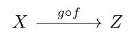

Note, it is an unfortunate mathematical convention to reverse the order of the arrows in writing composition. We call this standard order. Even though in looking at \(X \xrightarrow{f} Y \xrightarrow{g} Z\), \(f\) comes first, then \(g\), when writing their composite we write \(X \xrightarrow{g \circ f} Z\). This comes from the convention for writing function evaluation where we write things like \(f(x)\) or \(g(x)\) instead of \((x)f\) or \(x \circ f\). It would be better to write everything in diagram order, in which case we would write the composition \(f \circ g\). However, that would involve changing standard notation in too many places even for this stubborn author, so we will continue with standard order.

Back to deriving a suitable category definition, we can now put two compatible maps together to form a new map. The next condition looks at putting three arrows together. Consider

Now by the same logic from before we should be able to make a map from \(W\) to \(Z\) using \(f\) followed by \(g\) followed by \(h\). Composition concerns putting two maps together, not three. Given that, we have two ways to go from \(W\) to \(Z\) using \(f\), \(g\), and \(h\). Either first compose \(f\) with \(g\) to get \(g \circ f\), then compose \(g \circ f\) with \(h\), giving \(h \circ (g \circ f)\), where the parentheses indicate that \(g \circ f\) is the map composed with \(h\). The other option is to compose \(g\) with \(h\), giving \(h \circ g\), then compose with \(f\), giving \((h \circ g) \circ f\). So we could in theory have two maps from \(W\) to \(Z\) built from \(f\), \(g\), and \(h\):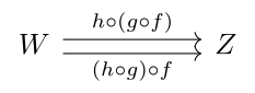

We will require these to be the same map, i.e. \(h \circ (g \circ f) = (h \circ g) \circ f\).

Only one condition remains. Every object \(X\) should have a relationship to itself by virtue of its existence. That is, if \(X\) is in our category (so it exists), we will require it to have a special identity map \(1_X\) which will correspond to doing nothing. Specifically, for every \(X \in \mathcal{A}\) we will require there to exist a map \(X \xrightarrow{1_X} X\) such that for any \(W \xrightarrow{f} X\), we have \(1_X \circ f = f\), and for any \(X \xrightarrow{g} Y\), we have \(g \circ 1_X = g\). The idea is that \(X \xrightarrow{1_X} X\) should leave \(X\) unchanged. We require it to exist for all objects, because, if an object \(X\) exists in our category, it should always be possible to map from \(X\) back to itself without changing anything.

We can now formally state our definition of a category.

Definition 1.2.2. A category \(\mathcal{A}\) consists of

• A collection of objects, and

• For every pair of objects \((X, Y)\), a collection of arrows / maps / morphisms \(\mathop{\mathrm{Hom}}_{\mathcal{A}}(X,Y)\), where, if \(f \in \mathop{\mathrm{Hom}}_{\mathcal{A}}(X,Y)\), we call \(X\) the domain or source of \(f\) and \(Y\) is the codomain or target of \(f\).

Subject to the following constraints:

• Composition: If \(f \in \mathop{\mathrm{Hom}}_{\mathcal{A}}(X,Y)\) and \(g \in \mathop{\mathrm{Hom}}_{\mathcal{A}}(Y,Z)\), then we can form \(g \circ f \in \mathop{\mathrm{Hom}}_{\mathcal{A}}(X,Z)\).

• Associativity: If we have \(W \xrightarrow{f} X\), \(X \xrightarrow{g} Y\), \(Y \xrightarrow{h} Z\), we require \(h \circ (g \circ f) = (h \circ g) \circ f\).

• Identity: For all \(X \in \mathcal{A}\), there exists \(X \xrightarrow{1_X} X\) such that for any \(W \xrightarrow{f} X\) or any \(X \xrightarrow{g} Y\), \(1_X \circ f = f\) and \(g \circ 1_X = g\).

1.3 Commutative Diagrams

Discussion 1.3.1. Already we have begun using pictures to describe things of interest. We are going to expand the use of these diagrams greatly in the rest of this book. Why? The use of diagrams will provide clarity to understand what is going on and efficiency of expressing what is happening. If objects are understood through maps into and out of them, diagrams are a clear, compact means of communicating about the objects and maps of interest in a particular situation.

Roughly speaking there are three equivalent ways of expressing the same mathematical content. First there are statements with words. We can describe what we mean, where if the words have unambiguous meaning in the context at hand then we know what we are talking about.

Next we have equations. Equations are statements saying two potentially different things are, in fact, the same thing or, as we will see later, at least equivalent in some way. Last section we began writing things like \(X = Y\) for two objects \(X, Y \in \mathcal{A}\) for \(\mathcal{A}\) some category. We also could have equality of maps. So we could have for \(f, g \in \mathop{\mathrm{Hom}}_{\mathcal{A}}(X,Y)\) that \(f = g\). In both cases “\(=\)” is notation that is shorthand for saying two objects or two maps are the same thing. Equations become compact ways of packaging certain statements. We can say the same thing with both, but we can say certain things more efficiently and unambiguously with equations.

Diagrams will do for equations what equations do for statements. Diagrams will be ways to package maps and, especially, equations involving maps into clear, compact pictures. We will end up seeing that a great deal (all?) of math is best done using pictures — a picture is worth a thousand words, as it were.

Definition 1.3.2. A diagram is a picture involving objects and arrows / maps / morphisms between those objects.

Discussion 1.3.3. We have already seen some diagrams last section. For example and are each diagrams.

Diagrams become particularly useful when we have multiple maps beginning and ending in the same objects. For example, consider the diagram 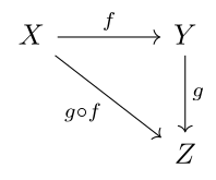In theory there are two ways to go from \(X\) to \(Z\) in the diagram. We could go via \(X \xrightarrow{f} Y\) and then via \(Y \xrightarrow{g} Z\) to go from \(X\) to \(Z\), or we could go \(X \xrightarrow{g \circ f} Z\). Now by definition \(X \xrightarrow{g \circ f} Z\) is precisely taking the first path, so the two paths are the same here. In other situations we will have paths through diagrams starting and ending in the same objects that need to be distinguished. Often our work will boil down to distinguishing whether different paths actually represent the same map.

Definition 1.3.4. A diagram commutes or is a commutative diagram if any two maps (including implicit compositions) with the same domain and codomain are equal.

Discussion 1.3.5. Let us immediately look at an example to get some practice with what this means. Say we have the following diagram 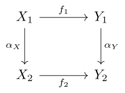There are four maps explicitly written: \(X_1 \xrightarrow{f_1} Y_1\), \(Y_1 \xrightarrow{\alpha_Y} Y_2\), \(X_1 \xrightarrow{\alpha_X} X_2\), and \(X_2 \xrightarrow{f_2} Y_2\). Since in a category composition of compatible arrows is always permitted, there are two implicit maps \(X_1 \xrightarrow{\alpha_Y \circ f_1} Y_2\) and \(X_1 \xrightarrow{f_2 \circ \alpha_X} Y_2\). The diagram above would commute if any maps (explicit or implicit) with the same domains and codomains are equal. The only such maps sharing source and target are \(\alpha_Y \circ f_1\) and \(f_2 \circ \alpha_X\). So saying the diagram commutes implies \(\alpha_Y \circ f_1 = f_2 \circ \alpha_X\). Conversely, if \(\alpha_Y \circ f_1 = f_2 \circ \alpha_X\), then the diagram would commute. So we see that the diagram becomes a way of saying the same thing as the equation, just in a different (usually superior) form.

What is so superior about the diagram versus the equation? First, the diagram exposes information that is easy to miss in the equation. In the equation you have to remember the sources and targets of all the maps. The diagram lists them right there plain as day.

A second, deeper reason is cross-context repetition. The same basic diagram will show up in wildly different contexts. Squares like what was just shown are important and ubiquitous. If we write things as equations we can miss this. Written as a diagram it can be easier to spot that something familiar is happening.

As an example — one that will at best make partial sense now — let us consider the naturality condition from natural transformations that we will see in two chapters. The equation form of these is \(\alpha_Y \circ F(h) = G(h) \circ \alpha_X\), while the diagram form is 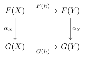This may look intimidating, but consider its similarities to the square just encountered They are very similar, and understanding what the simpler square says will make it far easier to understand what the naturality square says.

As a complete aside that the reader should probably ignore, the \(F\) and \(G\) are functors (topic of next chapter). One thing they do is map arrows \((X \xrightarrow{h} Y) \mapsto (F(X) \xrightarrow{F(h)} F(Y))\) and \((X \xrightarrow{h} Y) \mapsto (G(X) \xrightarrow{G(h)} G(Y))\). The natural transformation then is a way of mapping these image arrows \((F(X) \xrightarrow{F(h)} F(Y)) \mapsto (G(X) \xrightarrow{G(h)} G(Y))\) via maps \(F(X) \xrightarrow{\alpha_X} G(X)\) and \(F(Y) \xrightarrow{\alpha_Y} G(Y)\). We will cover all this shortly. Back to the main flow.

Discussion 1.3.6. The other major benefit of diagrams is that we can package many equations at once. As an example, consider the conditions defining identity maps. Fix some category \(\mathcal{A}\) and \(X \in \mathcal{A}\). There exists \(X \xrightarrow{1_X} X\) such that for any \(W \xrightarrow{f} X\), \(1_X \circ f = f\), and for any \(X \xrightarrow{g} Y\), \(g \circ 1_X = g\). \(1_X \circ f = f\) is equivalent to the following diagram being commutative 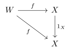and \(g \circ 1_X = g\) is equivalent to 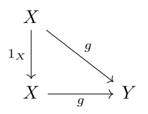being commutative. But we can put these together into one diagram 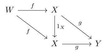The above diagram is commutative if and only if the identity map equations are satisfied. So we can use diagrams not just to clarify the maps involved or to spot commonalities across contexts, but also to compactly package multiple equations.

Remark. Remark 1.3.7. Importantly, the shape of the diagram does not change what the diagram says. What the diagram says is determined by the maps involved, not the way the maps are drawn on the page. So if both the following commute 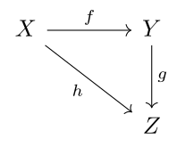and 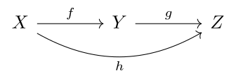then they are saying exactly the same thing. We pick shapes that we hope will help clarify, but do not confuse the shape of a diagram with the information it contains.

Remark. Remark 1.3.8. There is another related use of the term commutative that shows up frequently in math, and which we have already encountered in this text. For concreteness let us focus on addition on \(\mathbb{R}\) and multiplication of \(2 \times 2\) matrices \(\mathbb{R}^{2 \times 2}\). Addition on \(\mathbb{R}\) is a function \[\begin{array}{rcl} \mathbb{R} \times \mathbb{R} & \xrightarrow{\mathrm{add}} & \mathbb{R} \\ (x, y) & \mapsto & x + y \end{array}\] and multiplication on \(\mathbb{R}^{2 \times 2}\) is \[\begin{array}{rcl} \mathbb{R}^{2 \times 2} \times \mathbb{R}^{2 \times 2} & \xrightarrow{\mathrm{mult}} & \mathbb{R}^{2 \times 2} \\ (A, B) & \mapsto & AB \end{array}\] Each of these is a binary operation since they take in 2 inputs and produce one output. In the first example we say addition on \(\mathbb{R}\) is commutative since \(x + y = y + x\) for all \(x, y \in \mathbb{R}\). In the second example, multiplication on \(\mathbb{R}^{2 \times 2}\) is non-commutative, as \(XY \neq YX\) typically. (Please produce one such case yourself.)

In general, a binary operation on a set \(S\) is a function \[\begin{array}{rcl} S \times S & \xrightarrow{\mathrm{op}} & S \\ (x, y) & \mapsto & \mathrm{op}(x, y) \end{array}\] and \(\mathrm{op}\) is commutative if \(\mathrm{op}(x, y) = \mathrm{op}(y, x)\) for all \((x, y) \in S \times S\).

This notion of commutative is a special case of diagram commutativity for a particular diagram. Define the function \[\begin{array}{rcl} S \times S & \xrightarrow{\mathrm{rev}} & S \times S \\ (x, y) & \mapsto & (y, x) \end{array}\] a function that reverses the order of \(x\) and \(y\). Assume we have a binary operation \(S \times S \xrightarrow{\mathrm{op}} S\). Consider the diagram 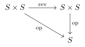We can see that this diagram commutes if and only if \(\mathrm{op}\) is commutative.

Discussion 1.3.9. The reader will need to become fluent in passing through the dialects of statements, equations, and diagrams. Luckily there will be lots of practice in the material ahead. We will begin defining many things in a diagram first way, although we will endeavor to make it clear what equation and even statement forms of the diagrams say. We are now ready to run through some examples of categories, some of which will make sense now, and others of which may not.